GEODEMO_4

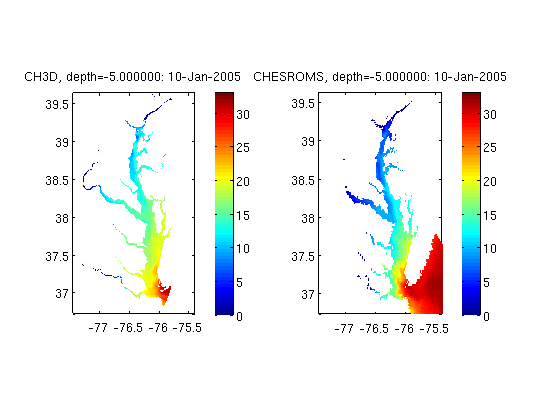
Compare horizontal slices from two different CF compliant structured grid models (CH3D and ROMS) at a particular time step and depth

Contents

CH3D

url{1}='http://testbedapps.sura.org/thredds/dodsC/estuarine_hypoxia/ch3d/agg.nc';
var{1}='salinity';
titl{1}='CH3D';

ROMS

url{2}='http://testbedapps.sura.org/thredds/dodsC/estuarine_hypoxia/chesroms_1tdo/agg.nc';
var{2}='salt';
titl{2}='CHESROMS';

dat=[2005 1 10 0 0 0];  % Jan 10, 2005 00:00 UTC
depth=-5;  % horizontal slice 5 m from surface
ax=[  -77.4572  -75.4157   36.7224   39.6242]; %lon/lat range
cax=[0 33];  %color range
lat_mid=38; % for scaling plots

Perform analysis without using dataset dependant code

Access datasets, get 3d field at given time data, interpolate data to a constant z, plot results at z depth

figure;
for i=1:length(url);
  nc{i}=ncgeodataset(url{i});
  jd{i}=nj_time(nc{i},var{i});  % using nj_time
  itime=date_index(jd{i},dat);
  disp(['reading data from ' titl{i} '...'])

  % using nj_tslice here, which doesn't allow for subsetting or
  % striding:  you get the whole 3D field at a particular time step:
  [s{i},g{i}]=nj_tslice(nc{i},var{i},itime);
  sz{i}=zsliceg(s{i},g{i}.z,depth);
  a{i}=subplot(1,length(url),i);
  pcolorjw(g{i}.lon,g{i}.lat,double(sz{i}));colorbar
  axis(ax);
  caxis(cax);
  title(sprintf('%s, depth=%f: %s',titl{i},depth,datestr(g{i}.time)));
  set (a{i}, 'DataAspectRatio', [1 cos(lat_mid*pi/180) 1000] );

end

reading data from CH3D...
reading data from CHESROMS...

Published with MATLAB® 7.13